Raymarching The Gunk
- Intro
- Game loop
- Overview
- CPU: From spheres to voxels
- Pipeline
- GPU: Generating the SDFs and clipmap
- GPU: Raymarching gunk to rendertargets
- GPU: Superimpose renders to GBuffer using material
- Unreal Engine integration
- Summary
Intro
In December 2021 we released a game at Image & Form and Thunderful called The Gunk. It was initially released for the Xbox Series S/X and Xbox One, followed by a Steam release on PC in the spring of the following year. The Gunk is a game about exploring an alien planet and clearing it of a corrupting slimy substance called Gunk. The player controls a space explorer named Rani. Equipped with a huge mechanical glove that can vacuum up all kinds of debris, she takes on the task of cleaning the planet of gunk and its corruption, which in turn also restores the lush vegetation of the planet.
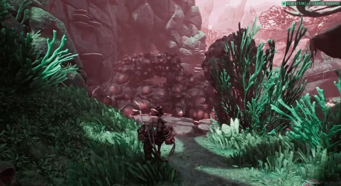
During this project I worked as the code lead and I was also responsible for developing the rendering tech for the gunk slime and its corrupting visual effect on the world.
For this game we wanted to clutter the world with gunk for the player to clean up. The gunk itself had to be easily placed by the team, and the player needed to be able to make dents and holes in it as well as remove it completely. The game had to be able to track the progress of cleaning and where gunk existed, not only on GPU for rendering, but also for the CPU in order to drive gameplay events and audio. We also discovered that it had to be very forgivable and able to automatically remove very small pieces of gunk on its own that would've been hard for the player to spot.
To achieve the wanted feel we decided to approach it by using volumetrics and see if that’d fit the bill. Volumetrics can be used to render clouds and fog, but also opaque surfaces. There are different methods to consider when rendering these kinds of surfaces: polygonal based marching methods, like Marching Cubes, are one route to take, splat-based surfaces another, and Raymarching yet another. The latter, in combination with Voxel based Signed Distance Fields is what we decided to explore. Raymarching is quick to get up and running and we wagered we could quite easily achieve pretty high resolutions by applying layers of noise to it.
And rendering something without using polygons felt very interesting to explore.
In this article I’ll break down the tech we created to get the gunk working and rendering in Unreal Engine 4 using a combination of compute shaders and the existing UE material pipeline, including the changes we made to the engine to optimize for async compute.
The solutions implemented and that I describe here stands on the shoulders of giants, I've gotten a lot of inspiration from some really impressive projects: especially the work done with Conetracing by Sebastian Aaltonen in Claybook, as well as the many different ways Alex Evans and Media Molecule approached SDF rendering in Dreams and the fantastic work done and taught on SDFs by Inigo Quilez.
Working on this tech was some of the most interesting work I’ve pursued so far, and it still holds lots of potential, so I hope it’ll be interesting to read about!
Game loop
In the game the gunk works like this:
- The player finds an area that is infested by gunk. The area around gunk is corrupted and grey and might spawn enemies and block paths.
- If the player moves into gunk they lose health.
- The player can absorb gunk, digging tunnels through it and removing it bit by bit. They need to scope their surroundings in order to find gunk in high- and low places, and around corners.
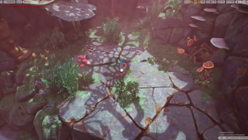
- When all the gunk is gone, the area kicks back to life: plants start growing and the area becomes lush again. The grey corruption effect on the vegetation and terrain fades away. New paths might open up.
Overview
I want to start with a brief overview of how gunk is authored by us in the Unreal Editor and the pipeline that then creates the data for it which the player can interact with and which is then used by the renderer.
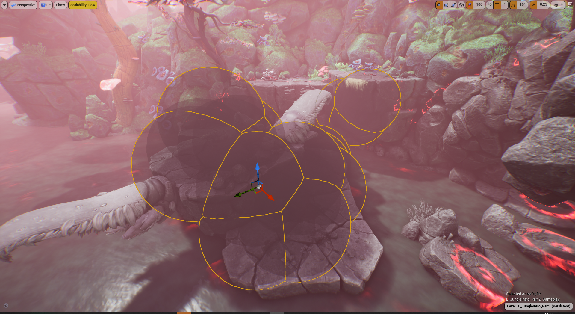 Sphere shaped actor based entities outlining an area of gunk in the Unreal editor.
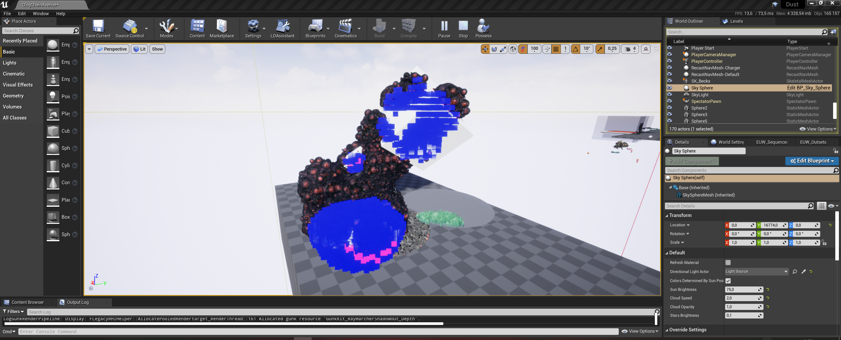
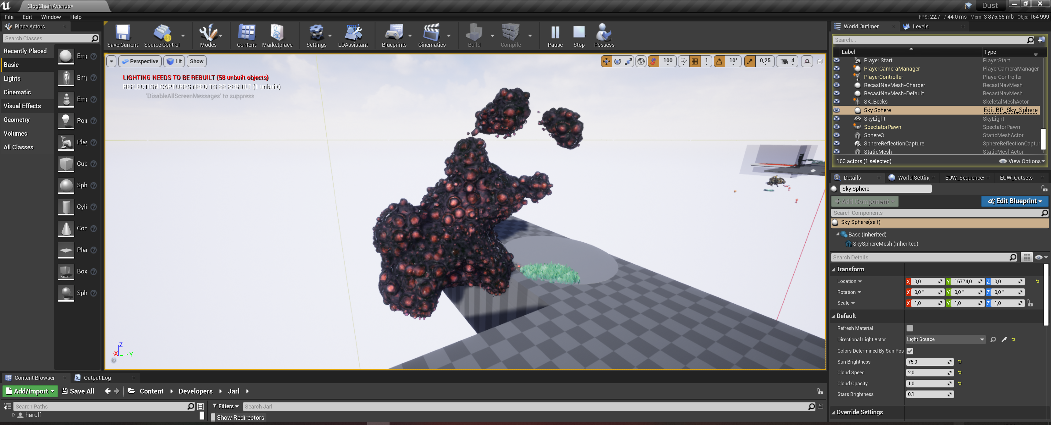
Before the game level starts, a set of sphere shaped Unreal actors are loaded that define where the gunk should be. These are placed in the levels by the level design team, like any other actor in Unreal Engine. Using regular Unreal Actors for placing gunk means that we get a non-destructive workflow for free. Actors can be moved, removed, undo'd, and scaled individually and in groups. A bunch of actors form the shape of an area of gunk. Designers can also visualise the final gunk shape while they edit the levels.
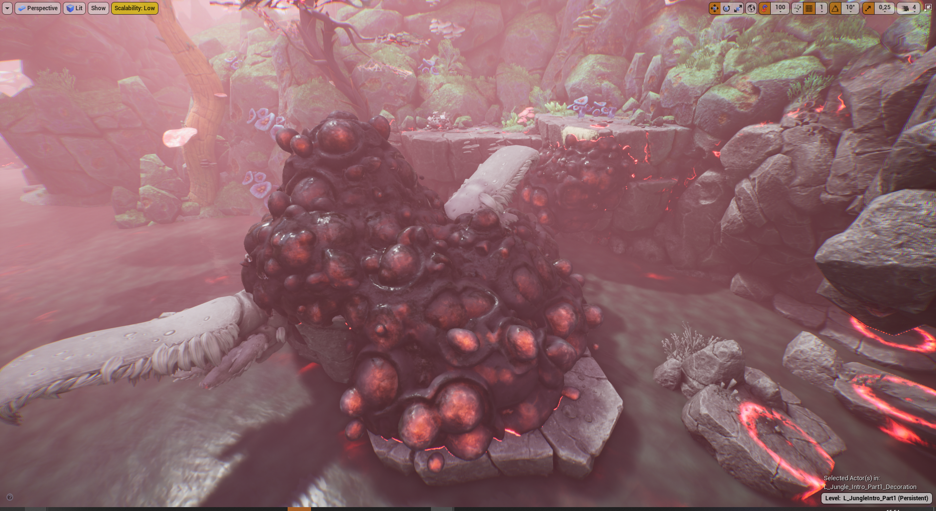
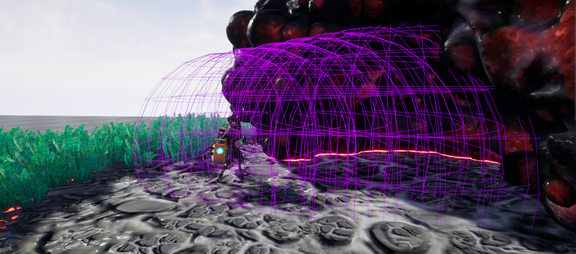
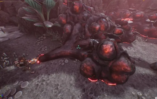
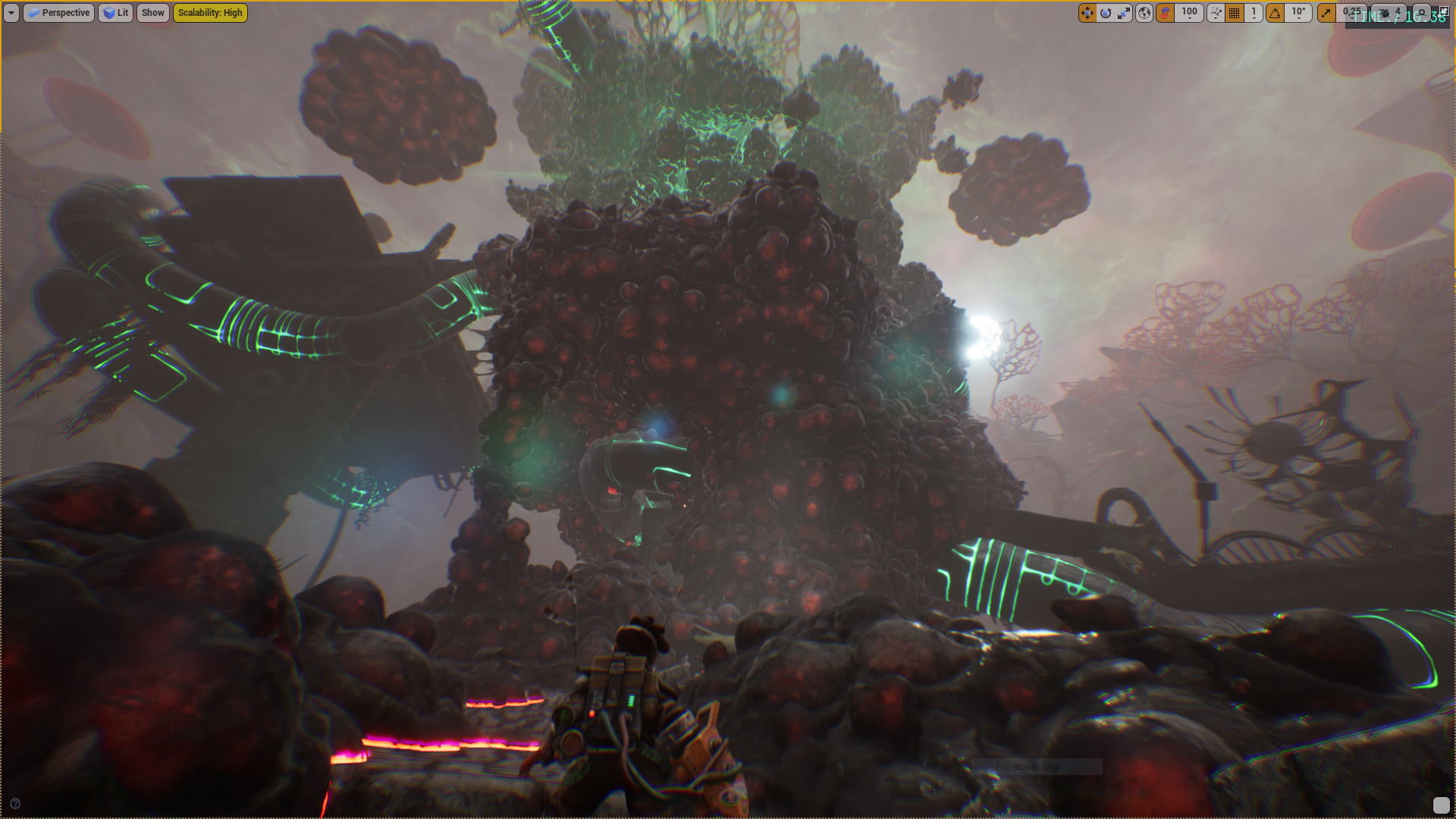
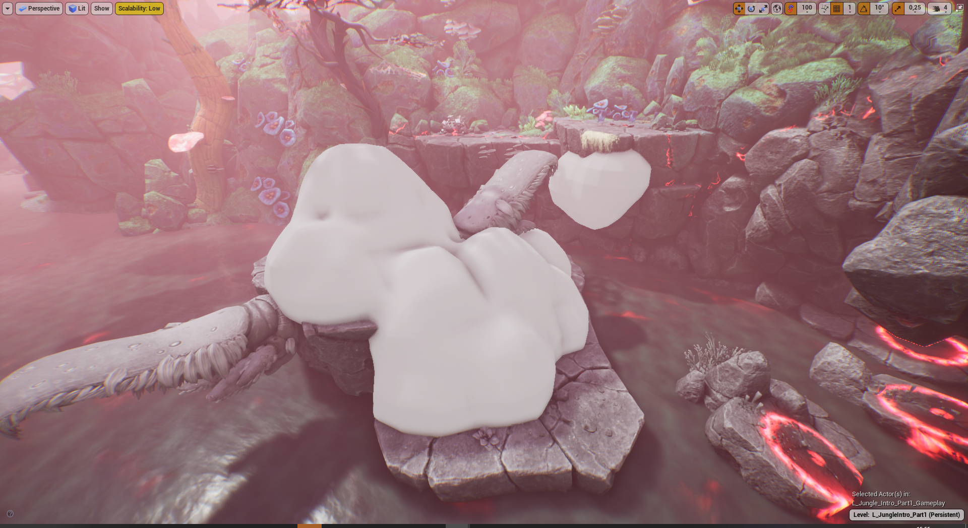 Raymarching gunk at its native resolution.
During game startup the gunk sphere actors are voxelized into fields of voxels. These are used for the game to look up how much gunk is left and where and also to handle collision against gunk. The voxels also serve as a basis for Signed Distance Field (SDF) generation, which is the data that we use to raymarch the surface. A lot of things happen in these steps, I'll dive deeper into these in a while! Just raymarching the field gives us the rough shape in the image above.
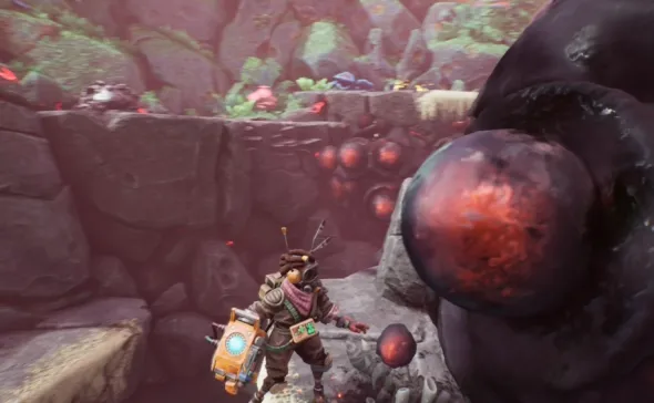
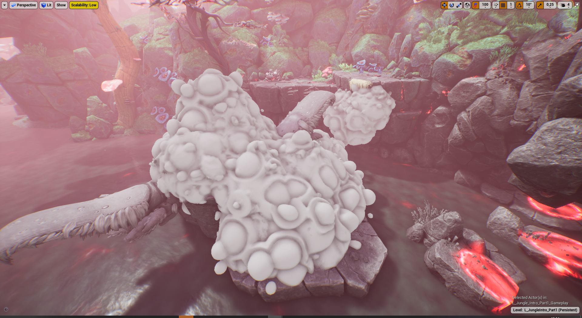 Raymarching gunk with added detail using noise textures.
To remedy the low chunky resolution we can apply tileable noise of different sizes. With some tweaking we can get it to hide the low resolution pretty effectively. This is a common trick for many 2d effects in games as well. We can also animate the noise easily and get that gooey, bubbly alien goop-look. Noise comes with its own headaches and issues for SDFs though. One big problem is that raymarching through the noise volumes as well as the base gunk volume takes more time per frame, but it allows us to have very coarse 3d grids for high perceived fidelity, which was good for us.
 Colouring is done through a regular Unreal Material.
When the surface is rendered fully, we render the results on screen using a full screen quad with per-pixel depth offset and thus we can apply a regular Unreal material graph on it and it will participate in the scene and react to lighting like any polygonal object. Note that this is possible with a slight tweak to UE’s default pixel depth offset calculation, which I'll go through later.
Sidenote: The grey corruption visible around gunk is a separate effect and system whose workflow is handled in a similar way. Designers can place actors to designate what should be corrupted around gunk. Corruption and gunk are then coupled together in game logic, so the corruption will fade away when all gunk in a corrupted area is cleared. The corruption effect acts on materials and blueprints and is actually not a post process, I should probably write a separate article on the solutions and optimizations involved in it.
That’s a rough overview of how we add gunk and what happens during gameplay. In the coming chapters we’ll dig deeper into the tech that drives each step!
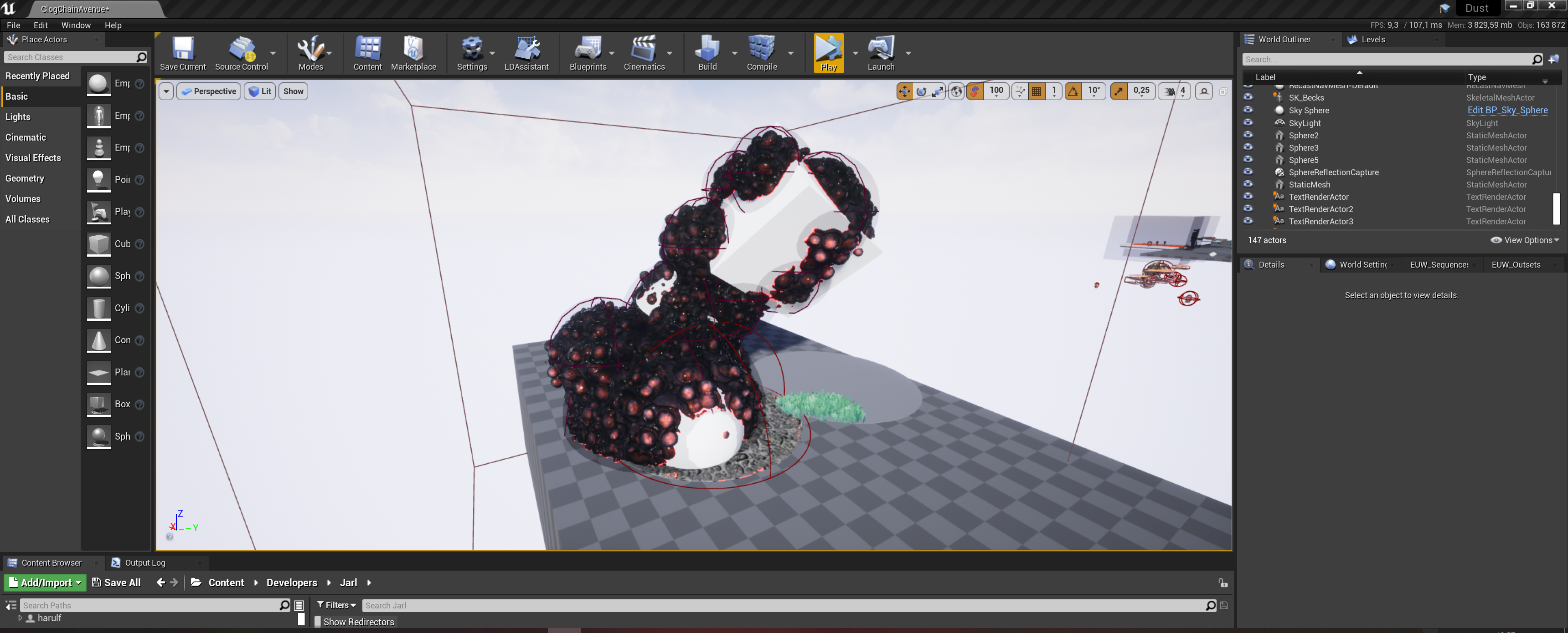
 Example of how gunk and the surrounding corruption is added to a level in Unreal using regular Unreal Actor objects. We've made sure to be able to render all our custom shaders in the editor as well. SDFs are recreated in the editor for each edit so we don't need to serialize them.
CPU: From spheres to voxels
On the CPU side we process the sphere actors into volumes of voxels which we can keep track of during gameplay. They are also what the player interacts with. They are way coarser than what we render in the end but their resolution are enough for the kind of interaction and collision detection that we do in this game.
Gunk voxels
We group the sphere actors into logical gameplay areas. We can use these groups to drive gameplay events, and handle distance culling per group and we also use them to create the volumes for the gunk, the first step here is to voxelize the spheres. Think of the groups as the canvas on which we add voxels based on the spheres. The groups in turn keep track of the amount of active gunk voxels left in them.
Voxels are a handy way to represent densities in 3d. They are essentially cubes in a 3d grid.
 Voxels visualized on top of gunk being absorbed. Voxel "HP" shown as square in the middle, bigger=more.
The grid of voxels is coarse and the voxels are big. We want to try to keep the grid as coarse as possible so we don’t require as many voxels and not as much memory. But we still need the voxels to be small enough so we don’t get too blocky or pointy gunk shapes.
Voxels in the gunk are represented by single precision floats which represent “health points” for the voxel. This is used to tweak the absorption speeds that we want but also used to help with volumetric anti aliasing in the generation of SDFs. The default HP for a gunk blob is lower at the outside edges.
 A gunk blob's voxels seen from above. To the right is what our blobs look like if the HP would be plotted as a grayscale value, as opposed to a binary representation to the left.
Mesh cut-away
Gunk must not be spawned inside level geometry, like floors and walls. However as we use a sphere shaped actor to define a blob of gunk, we need to consider that they might overlap with level geometry. The solution we opted for to remove gunk inside geometry is to voxelize geometry inside the gunk areas and use them to subtract the gunk voxels. This system could’ve been utilised in the reverse also, to place gunk using meshes, although we never got around to try that.
The level is voxelized by raycasting over a 2d grid of voxel columns, top to bottom, and finding all entry and exit points along the line.
This operation is only done once per level load.
 Test showing various geometry intersecting the gunk. The ground plane as well as some white meshes.
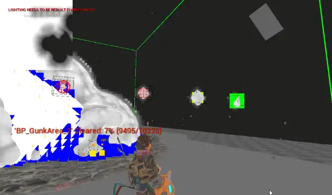
 When the game starts the gunk that is intersecting with geometry will be cut away, as indicated here by the blue debug plots.
 If we delete the geometry we can see that the gunk was cut away there.
For landscape actors, which are used in many places in the game, we decided to let the system regard them as being of infinite thickness below the ground level. We could take that shortcut, as we didn't use overlapping landscapes, or landscapes above caves.
Player interaction
Absorbing
The player can absorb gunk. Behind the scenes this essentially means that the player can subtract spheres of gunk. These spheres are aligned to roughly approximate a cone shape, for which we can change the segment sizes of. We do occlusion checks into the gunk along the cone direction, and make segments inside gunk smaller, to make sure that only the surface of gunk is being removed. This occlusion check queries the gunk voxels on CPU to determine if each cone segment part is inside gunk or not, and that affects each segment removal strength. We used this to tweak the speed of absorption and its distance- and density effectiveness.
Where voxels have been absorbed we then spawn particles that move from the gunk blob to the nozzle of the absorb glove on the player. These particles are also rendered as gunk, more on that later.
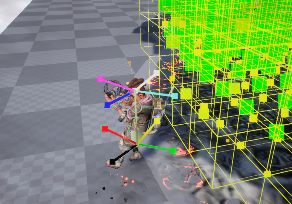
 Absorb cone visualisation. Upper image shows the absorb cone overlapping with Gunk. In the lower image the gunk renderer is switched off to show how the absorb cone is scaled down in size if it is inside Gunk, to simulate how the Gunk absorber absorbs the nearest Gunk first.
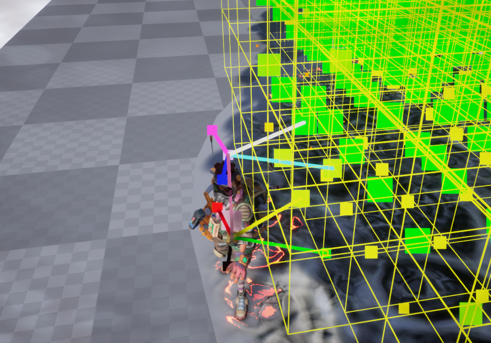
 Here the player has absorbed all gunk within the cone influence, here we can see that the cone is now at full scale since it has no gunk blocking it.
Overlap detection
All collision checks with gunk are done by checking overlap with voxels. The player will take damage if they come into contact with gunk. We did experiments with generating distance fields on CPU and also some early experiments with readbacks from GPU (when the game was 2d based). But just checking the voxel data is good enough for our game so we could keep the overlap detection system pretty simple in the end.
To make the overlap detection feel like it's done on a smoother surface we do trilinear interpolation of the nearest voxels. Here the antialiased nature of the HP of the voxels also help to make it feel a little smoother (see Gunk voxels).
 Visualisation of trilinear interpolation outside and inside voxels.
Trilinear interpolation is a method to get an interpolated value from a 3d dataset. It is essentially the interpolation of two bilinear (2d) interpolations. It works by sampling the 8 neighbours around a point and use the fractional values of that point's normalized coordinates in relation to the neighbours to linearly interpolate between them. First interpolate two parallel axes both in the top- and bottom plane of the neighbourhood (1d, linear interpolation). Then interpolate between their results using the axis connecting those lines (2d, bilinear interpolation). Then interpolate between those results on the axis connecting the two planes (3d, trilinear interpolation). In the images above you can see a line visualization of it drawn on top of Rani.
Sound ambience
Keeping voxel data on CPU also helps us generate sound ambience when the player is near gunk. And this ambience and where and how it plays changes along with how the gunk's shape is changed when the player absorbs it. My colleague Magnus Martinsson implemented the system which took the voxel data as input and transformed into something useful for the FMOD sound engine.
Cellular automata
An issue we ran into early was that players missed spots of gunk when cleaning. Something which was made worse by the fact that the gunk is animated by additive/subtractive noise (so a voxel can get animated away for a while). We tried to make the noise as tight as possible to the original gunk shape, but we couldn’t trade away too much of the fidelity it provided. To remedy this we run a cellular automata on the gunk field. Its rules dictate that single gunk voxels without any neighbours, or clusters of gunk voxels with low collective HP should shrink and disappear.
As we have HP on the voxels we can shrink them away gradually and individually. With a lot of tweaking this system helped us quietly and sneakily clear up small specks of gunk that the player might miss.
Cellular automata was something we explored several times during development. At one point we used it to auto-regenerate gunk so that it would flow outwards from existing clumps and fill up what was once absorbed.
Gunk particles
The stream of gunk that is created when absorbing is particle based and built using a custom (and very simple) particle system written in C++ that controls the particles.
Particles are small position+velocity structs that we update each frame. They are pulled towards Rani’s glove as well as the centerline of the absorb cone. This gives us a neat vortex effect. When particles are near enough, they smoothly interpolate towards Rani’s glove position, regardless of previous speed, to make sure they never miss the nozzle.
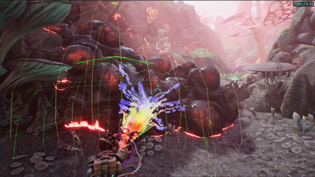
 Debug of particles. Each blue dot draws an SDF onto the transient render target. The lines near the nozzle visualizes particles that are near enough to switch to a simple linear interpolation towards the target (so that they never miss).
Then each particle renders the signed distance function for a sphere to a 3d render target. We don’t do any voxelization for these as we don't need to keep track of the volume on CPU in the same way as the gunk areas.
Pipeline
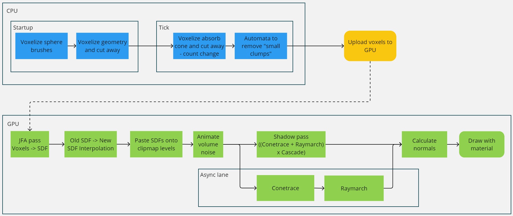 Overview of each step getting gunk rendered to screen.
GPU: Generating the SDFs and clipmap
Voxels to distance field using Jump Flood Algorithm (JFA)
Voxels are sent over to the GPU as a buffer of floats along with volume dimensions. But to render the voxels as a smooth surface in the raymarcher we need to first create a distance field from them. Our SDF generation pass creates a new volume in which each cell has a value that is the distance to that cell’s closest surface. There are several different ways to achieve this. A naive approach would be to check the distance to each cell and select the shortest, for each cell. That would be very slow. A popular algorithm that speeds up this process is the Jump Flood Algorithm (JFA), it's pretty clever and fast! It's perfect for the GPU so we implement it as a multi-pass compute shader that takes voxels as input and outputs a distance field volume texture.
JFA steps
- We start by creating a new volume where, for each cell, we write the coordinates of that cell if it is on the surface of the volumetric shape. How the surface is determined can be done in many different ways, the way we do it is by calculating a gradient over the cardinal neighbours. If the gradient has magnitude there is a surface.
In JFA, this is called the “seed” pass and it is from which we can “flood” the remaining pixels with info.
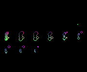 Seed volume created from a volume of gunk voxels, represented here as a 2d array of slices.
 - JFA will then run a pass until a step size is 1. The step size is initiated to half the size of one axis of the volume. For each pass of JFA the step size is halved. Thus the amount of passes needed is log2(axis size).
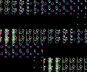
 JFA passes, each using the previous as input.
 - For each step in a pass, each cell checks its neighbour in each cardinal- and diagonal direction at a distance the length of the current step size. The cell gets the closest coordinates stored on one of the checked neighbours. As the step sizes decrease for each pass the values will continue propagating and we will eventually end up with a completely filled volume, where each cell has the coordinates of its closest surface cell (a seed cell).
- In a final pass the distances from each cell to its stored coordinates are calculated. If the cell is also overlapping with a filled voxel from the original buffer, then we know the distance is inside so we flip it (ie. flip the sign, utilising it as an is-inside flag, making it a signed field), a simple way of differentiating inside and outside distances. The end result is our signed distance field. This field now contains the distance to the nearest surface for any cell.
 The SDF generated by calculating the length of the vectors of each cell in the JFA buffer.
Antialiased seed value
It is also worth noting that we modify the seed pass of JFA a little. We want to utilise the anti alias property of our voxel, ie. their HP in order to get smoother surfaces. With regular JFA, a cell writes its exact coordinates, but nothing stops us from tweaking this value to better fit the surface, so we tweak it to get sub-voxel precise coordinates which are then propagated as usual in the next passes.
In our case we experienced the best results when doing it like this:
- When creating the seed value, we use the gradient if the cell is empty and the gradient has magnitude. This will create a seed outline outside all non-empty voxels.
- The gradient tells us the difference in density between the outside and the nearest filled voxels. It also tells us the direction, in our case it will point in towards more dense voxels. We want more dense voxels to push the edge further out and less dense voxels to pull it further in. This will make it possible to have one voxel blob that scales, and to have the gunk surface retract slowly when absorbing.
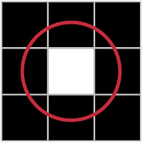 Filled voxel (white) and the effective surface edge (red) we want for it.
We approach this in such a way that the surface for a completely filled single voxel will render as an approximation of a sphere, overlapping other cells slightly.
Filled voxel (white) and the effective surface edge (red) we want for it.
We approach this in such a way that the surface for a completely filled single voxel will render as an approximation of a sphere, overlapping other cells slightly. - For empty voxels, the offset to the surface is given by the gradient of neighbouring voxels. If the gradient has a size of 1, it means the nearest voxel is full. So the offset should be 0, as we then want the edge on the middle of the current voxel (this achieves the slight overlap mentioned in step 2):
float3 SubVoxelOffset = GradientDirection * (1.0f - GradientLength);This furthermore means that if the voxel is less dense, say 0.25: then the gradient from an empty neighbour also becomes 0.25. So in that case we want the edge further inward from our current empty voxel: 1 - 0.25 = 0.75 voxels away inward. This excellent article by Ben Golus explains this even further and his 1D visualizations are a great way to showcase this, so I've used a 1D visualization below as well: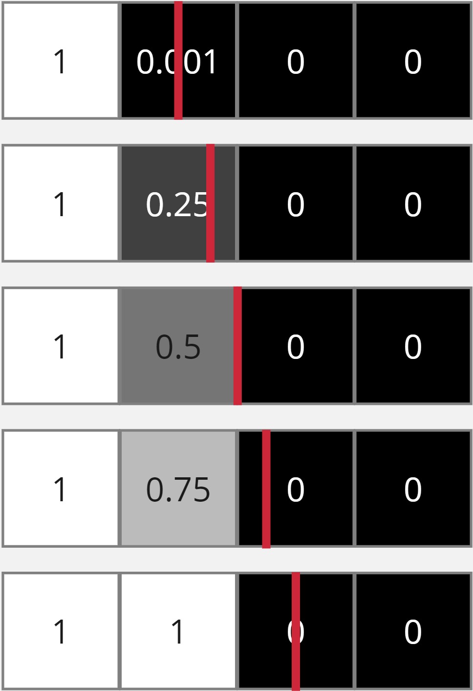 Effective edge (red line) placement based on partial voxel values.
 Single voxel test with different HP values and anti aliasing on the JFA seed values. Effectively allowing us to scale individual voxels as well as smoothing edges.
SDF interpolation over time
The JFA update pass is run when the gunk voxel field is modified. The anti aliasing measure makes the surface smoother than without, but the low resolution on the voxels still rears its ugly head when the player absorbs gunk from its surface as the SDF changes between old and new with some visible discrete stepping artifacts. We also need to smooth changes over time! In order to remedy this we continuously interpolate towards the newest SDF from the previous frame’s SDF.
Clipmap
At this stage we could start raymarching the volumes, and this is what we did for a while during development. However, if the amount of SDFs and the draw distances vary a lot the performance might fluctuate too much. In order to even it out we draw the SDFs onto a volumetric clipmap first. The clipmap has three levels of detail, so SDFs farther away are drawn onto a canvas with lower resolution, while the SDFs closer to the camera are drawn at their natural resolution (or higher to get a little smoothing using hardware interpolation).
SDFs are drawn onto the clipmap only when the clipmap moves. The clipmap moves in large discrete steps to lessen the amount of times it needs to update and to not get aliasing/flickering. The clipmap's position is aligned with the camera:
 Clipmap visualized in 2d. Low resolution at the farthest level with increasing effective resolution the closer we get to the camera. As each level scales they have roughly the same internal resolution, but cover different distances in world space.
The clipmap blends the LOD levels with linear interpolation so the transition is less visible.
Now we have a volume (with 3 LODs in the form of clipmap) that represents the gunk volume in the scene. But it is rough, we need to add detail noise at a higher resolution than any of the clipmap levels.
Noise animation pass and asset authoring
Before rendering the gunk clipmap, we run a noise animation pass. We want to animate all noise into a tileable texture that we can sample during raymarching. For the noise calculations we ran this was a performance increase for us, compared to running the noise calculations in the raymarcher. In our case the amount of noise calculations during raymarching would be more (screen size x * screen size y * steps) than for our noise volumes (128 * 128 * 128). A volume of constant size is also nice as it has a more constant cost that doesn't fluctuate as much. You do sacrifice noise resolution however, as sampling a texture in the raymarcher is not cheap either.
Noise editor
The animated noise is made up of several other noise textures that interplay and give us the bubbly texture of gunk. Each noise texture is a static volumetric texture and they are created in Unreal, using material graphs.
I set up a system where a material graph is used to create volumetric noise. An editor utility widget is then used to bake this noise to a texture. Combined with a preview level we can create and preview the noise and render it to a texture pretty easily. The tool is somewhat of a bodge but it works. Had it needed to be used by more developers it would have needed some more love, or just having us invest in a dedicated tool.
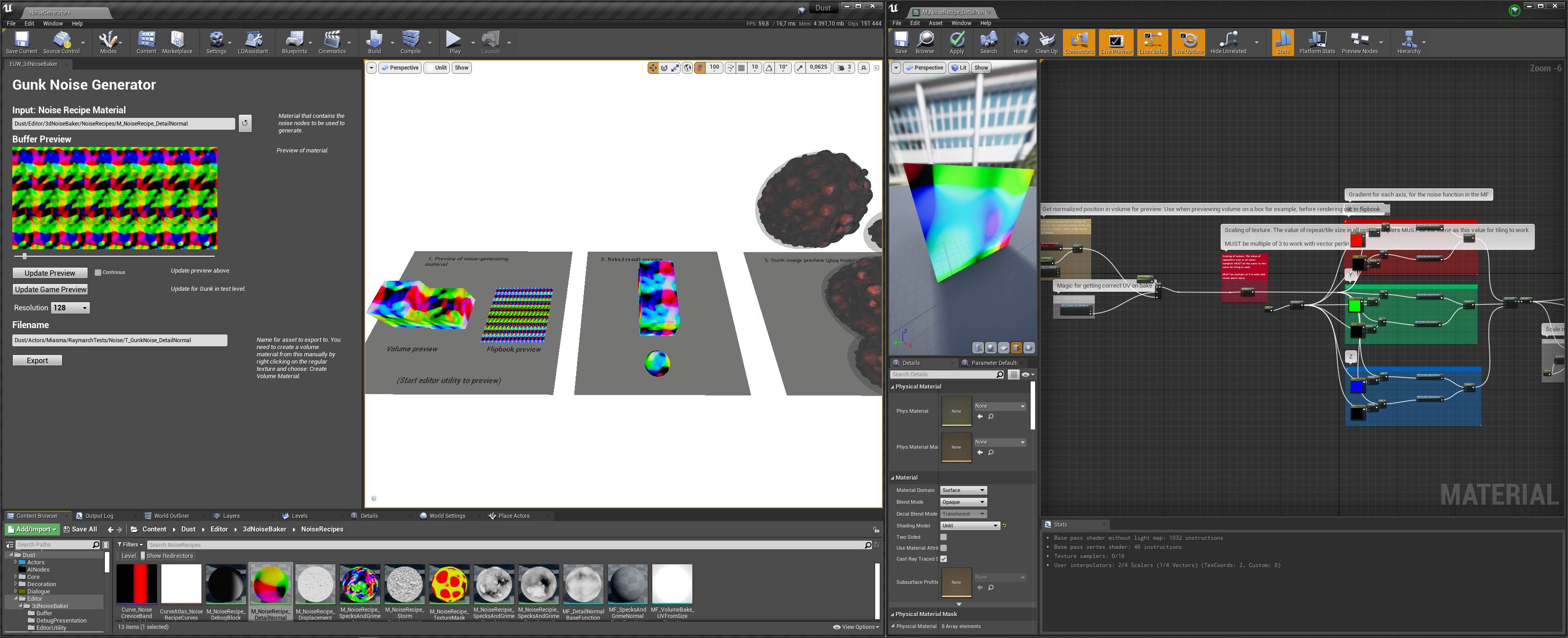 Custom noise texture renderer which can render and bake volume texture noise defined using materials. Implemented using the very handy Editor Utility Widget system in Unreal.
During runtime a compute shader then samples all our noise textures and animates their UV (some using previously sampled noise as offset), multiplies them together and outputs to a volume render target.
Animation looping
Care needs to be taken to the time offset used for sampling the noise, when it gets too large we get float precision artifacts in our noise. This is uncommon to occur, but we still don’t want gunk to glitch out if you leave the game running on a level for a few hours. To remedy this, the time and noise animation is made to loop. To get it looping, without having to place restrictions on timing variable multipliers (to avoid popping), we do a crossfade interpolation from the current state towards time 0 after a set amount of time. This requires double the samples during transition, so we want to do this seldomly. Like every hour into a level max, for a couple of seconds. When near our animation end: sample a value approaching zero from negative, then, when at zero, we get a perfect transition to restart.
const float3 UV = float3(ThreadId) / (float)OutNoiseSize;
const float a = fmod(Time * TimeModifier, LoopTime);
float Noise = CalcNoise(UV, a);
if (a > BlendStart)
{
    Noise = lerp(Noise, CalcNoise(UV, a - LoopTime), (a - BlendStart) / BlendTime);
}
OutputDisplacementNoise[ThreadId] = Noise;
GPU: Raymarching gunk to rendertargets
Raymarching is a way to render volumes, it works by stepping into the volume until a step has passed a threshold value. This is done for each pixel to be rendered. Raymarching is commonly used in games nowadays to render clouds and wisps of fog. For transparent rendering, like clouds, raymarching will accumulate density values along its step. In the gunk we treat the gunk as opaque so when we hit the surface we output the pixel depth immediately.
The way a step size is determined in raymarching can differ. As we have distance values per voxel from our SDFs, we use them to determine the step size. This helps us keep the number of steps down, which is important for getting raymarchers running fast. Amounts of steps per pixel is the biggest performance bottleneck for these kinds of algorithms, as they cause the shader to become too sequential and hinders parallelism due to threads having to wait for each other.
For each iteration we find out what the current shortest distance to the surface is and step that far forwards, which is safe. If the step took us inside a surface (negative distance) it means that the nearest surface was hit. If so, we return the result, otherwise we keep stepping given the next distance to the closest surface. This is repeated until a surface is hit or we have stepped outside the volume bounds. This variant of raymarching is also called sphere tracing.
For the gunk we define the threshold for a surface to be the size of a pixel's spherical bounds at that distance from the camera, given the view projection. This can be referred to as cone tracing, we use this even more extensively in a pre-pass which I'll get into soon.
 Tracing from the camera to the gunk surface using the SDF to get the next step size to the nearest surface. Distance compared to the screen pixel's coverage to determine if a surface was hit.
Simplified, the core raymarcher looks something like the code below. On the CPU we calculate a scale factor of a pixel's size along the depth of the camera frustum, so we can use it to determine when a pixel intersects a surface:
// Ratio of diagonal to a side of a square.
static constexpr float UnitHypothenuse = 1.41421356237f;
// How much view area scales in world by distance due to FOV angle.
const float FOVScale = FMath::Tan(HalfFOVRadians);
// Size of a pixel in world on the camera origin. Viewport is 2 units wide (-1 to 1).
const float PixelSizeWorldSpace = (FOVScale * 2.f) / (float)RenderTargetSize.X;
// How much the radius of a circle encompassing a pixel is, depending on how far away from the camera it is
ShaderParams.PixelConeRadiusByDist = PixelSizeWorldSpace * UnitHypothenuse * 0.5f;
This is one of many parameters sent along to the shader. Then inside the shader, the clipmap levels are iterated and each are marched through until something is hit. For each clipmap level its volume texture is marched using a function similar to the simplified one below (without optimizations):
bool RayMarchClipLevel(float3 RayOrigin, float3 RayDir, inout float RayDist, float MaxDist,
                       Texture3D<float> ClipLevel, float3 ClipCenter, float ClipSize,
                       out float3 OutPoint, inout int Iterations)
{
    float SurfDist = 0.f;
    for (int i = 0; i < MaxSteps; ++i)
    {
        ++Iterations;
        // Step to next point in world space.
        RayDist += SurfDist;
        if (RayDist >= MaxDist) return false;
        const float3 Point = RayOrigin + RayDir * RayDist;
        const float ConeSegmentRadius = (RayDist + NearPlane) * PixelConeRadiusByDist;
        // Get world space distance to nearest surface.
        SurfDist = SampleGunk(Point, ClipLevel, ClipCenter, ClipSize);
        if (SurfDist < ConeSegmentRadius)
        {
            // Hit if pixel, as projected at this distance, intersects surface.
            OutPoint = Point;
            return true;
        }
    }
    return false;
}
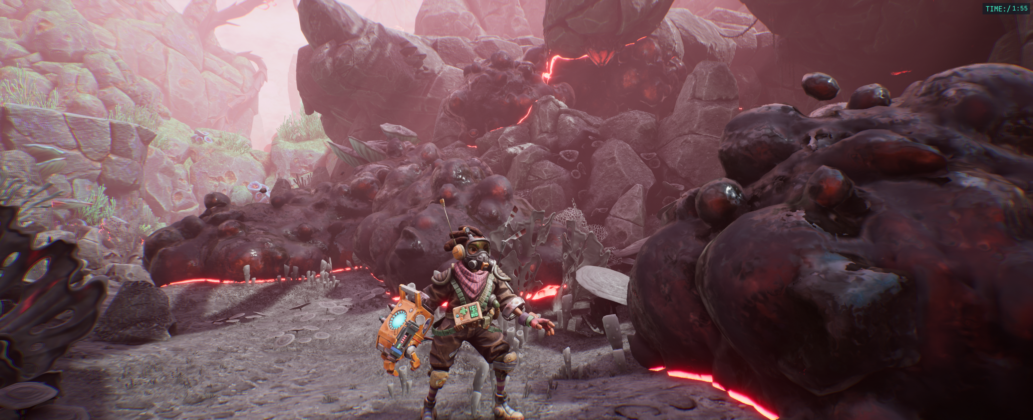
The function call to "SampleGunk" samples the texture at the given point. It also applies details that we want on a per ray step resolution, like detail noise texture sampling, particles and the camera hole function. The value "Iterations" is very handy to use and output to its own channel in the render target in order to gauge what areas needed the most steps, either as is or in some other fashion, like a heatmap.
Stepping through clipmap with blending
As our final SDF that we step through is layered in the form of a clipmap, we start by stepping through the nearest clipmap and continue through the following until a surface is hit. A line-AABB test is used to find the start point on the clipmap level's surface. The clipmap levels have roughly the same texture resolution each, but differ in world size. That way we are effectively sampling max 3 base shape SDFs per pixel and we get a lower level of detail farther away where we don't need as much detail.
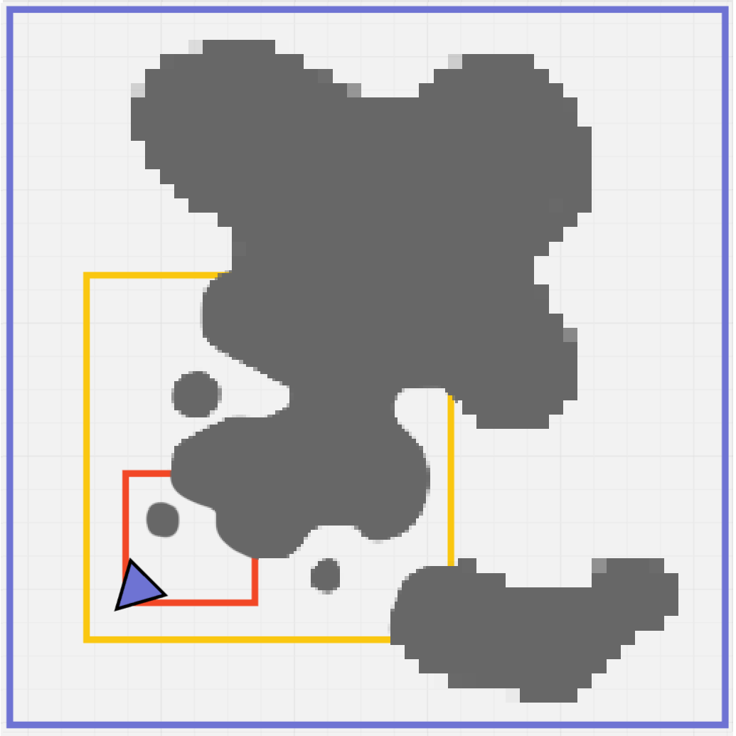
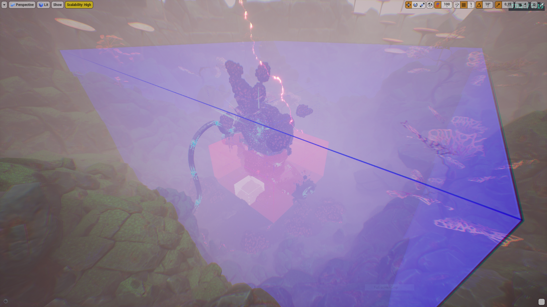 Clipmap levels. Level nearest player = White box. Middle level = Red box. Far layer = Blue box.
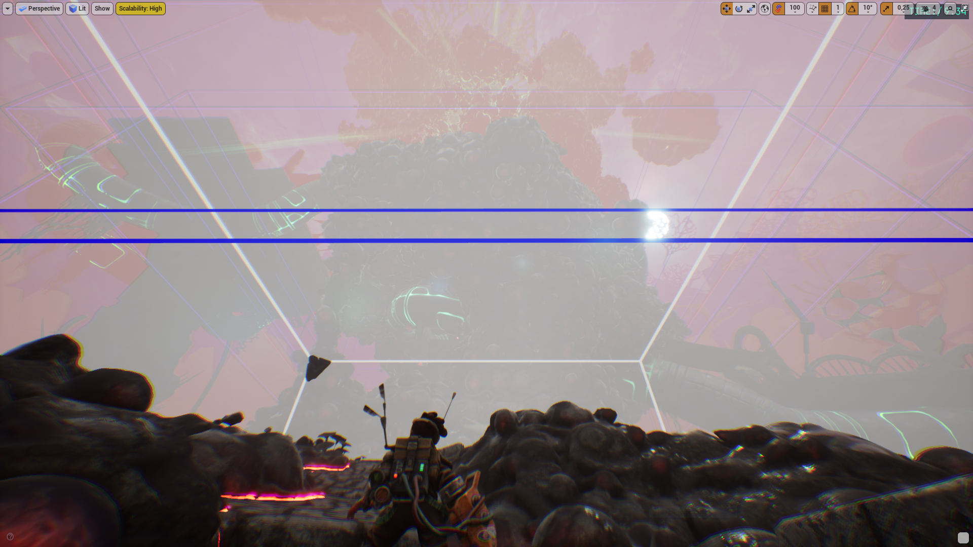 The same clipmap as seen from the player's point of view.
 The full rendering without debug visualization of the levels.
To avoid popping near the borders of the clipmaps, we sample both levels there and interpolate the result based on the travel distance through the border.
For each sampling in the clipmap level’s volume texture we also add the animated displacement noise to the distance to get the wobbly and noisy surface on the gunk. This unfortunately lessens the “euclideanness” of SDFs, making the distances not as correct which will lead to artifacts. We compensate by scaling down the step size by a constant factor which looks good for our noise. This is a big drawback for noise layering and other distortions, as it increases the steps needed on top of the extra sampling. On the other hand, as mentioned, noise diffuses the low resolution of the base SDF, so it is a bit of give and take.
Particle- and camera hole layers
In the last steps during the raymarching sampling, we then union the sampled clipmap level's distance with the transient particle effect layer’s SDF (see Particles). The transient effect layer is unioned after noise is applied and thus does not get any noise, but will blend into the noisy surface. This is how we get the absorb stream to be slick and smooth and give the appearence of the gunk being more fluid when absorbed.
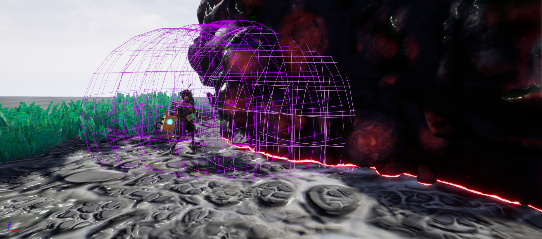
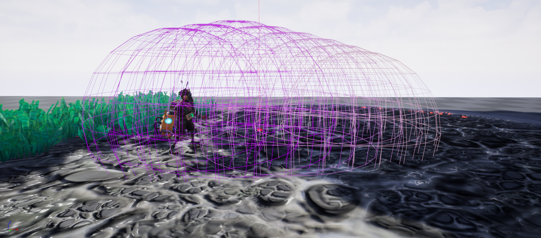
Another transient effect is the "camera hole" which is subtracted from the final distance after the particles sampling. On high spec targets, like Xbox Series X, we render it as a signed distance function of a capsule. This gives a much crisper per-pixel outline to the camera hole, but it is unfortunately a little too expensive on lower spec hardware. So on lower spec hardware, like the Xbox One, we subtract a low resolution, baked sphere SDF texture to save on performance.
 Subtraction of gunk temporarily around the camera, to keep the player visible
These are the base steps to get the per-pixel intersection information of gunk which we can use for depth, normal and texture information. However, just raymarching into the scene from the camera position is too costly. We want to lessen the amount of steps needed to reach the surfaces. The fewer steps we have, the less math and texture samples we have to do.
Bounding box test
One simple way of shaving away lots of empty space is to do bounding volume tests first. We can do a line-box test for each pixel to each bounding box of the gunk SDFs. And then use the hit location of these as starting points for the raymarch. This works well for gunk far away from the camera and from each other, but as soon as we get up close we still have too much empty space to traverse.
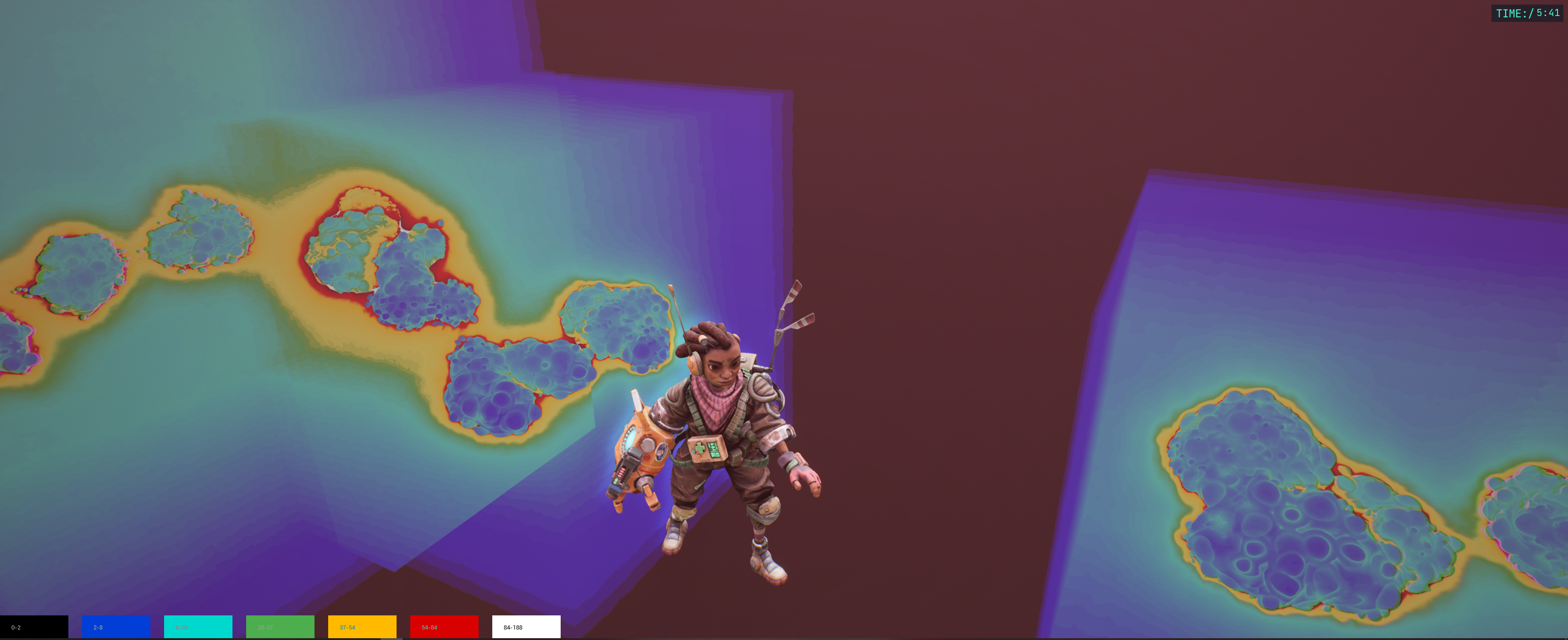 Axis aligned bounding boxes visible using a debug heatmap visualization. It shows how many steps were needed to reach the surface or stop the marching. Cooler colours mean fewer steps. Black means that only bounding box tests were made.
Low resolution conetracing pre-pass
In order to get even tighter ray starting points we perform a coarse cone trace pass before the raymarch pass. At an 1/8th of the final resolution we trace a cone into the scene. The cone scales linearly with the camera frustum, in that its section at a distance represents what size a pixel would have at that distance from the camera to exactly cover a pixel (sphere bounds, with diameter = pixel diagonal) on the screen. Since the cone trace resolution is 1/8th of the final resolution, its pixels can be seen as tiles that cover 8x8 pixels of the screen.
Tracing a cone which expands in this manner means that we get end results that won’t intersect with the surface. In our case this is a truth with modification though, due to our noise displacement of the field, which requires very fine tuning of step parameters to lessen risk of visual artefacts. Without noise it is pixel perfect however. The cone tracing algorithm is very similar to spherical raymarching. But instead of comparing the distance and whether it is less than zero, we compare it to the radius of the cone segment at that step. If the distance is less than the radius (plus some error-margin for the noise) we store the previous result.
Since we now do this rough evaluation as a pre-pass to the raymarcher, we no longer need to do AABB tests in the raymarcher, we only do it in the conetracer to get good start values.
We store entry, exit, 2nd entry and far bounds in a render target. We store the first exit in case the hit is on an edge and the ray in a tile might not hit a surface. If so we then know that the ray is safe to teleport to the 2nd entry when it has passed the first tile exit. Thus we can skip at least one more area of space behind the first hit. The far bounds are stored in order to determine when the ray has exited the last SDF bounds and can’t hit anything more. This way we don’t have to do another AABB test per ray. The first releases of The Gunk had a bug which caused the shader to not be able to do this exit bounds test, and thus those shaders were a lot more expensive (about +2 ms on Xbox Series X and +4 ms on Xbox One), this was later fixed in a patch.
 Conetrace buffer at 1/8th of screen resolution per axes, storing the first entry point in R, first exit in G and the second entry point in B.
So in short, we really want to minimize the amount of steps needed per pixel and in order to do that we want to skip as much empty space as possible. This is done in steps, first by finding the closest bounding box surface using a line intersection test. Then we trace a cone from there using the distance field. It gives us a tight starting point as well as some more info on what lies ahead. Using this we can run the final fine granularity raymarch and skip lots of empty space. Doing all of this allows us to render it all in about 4 ms instead of 20 ms.
 Final render
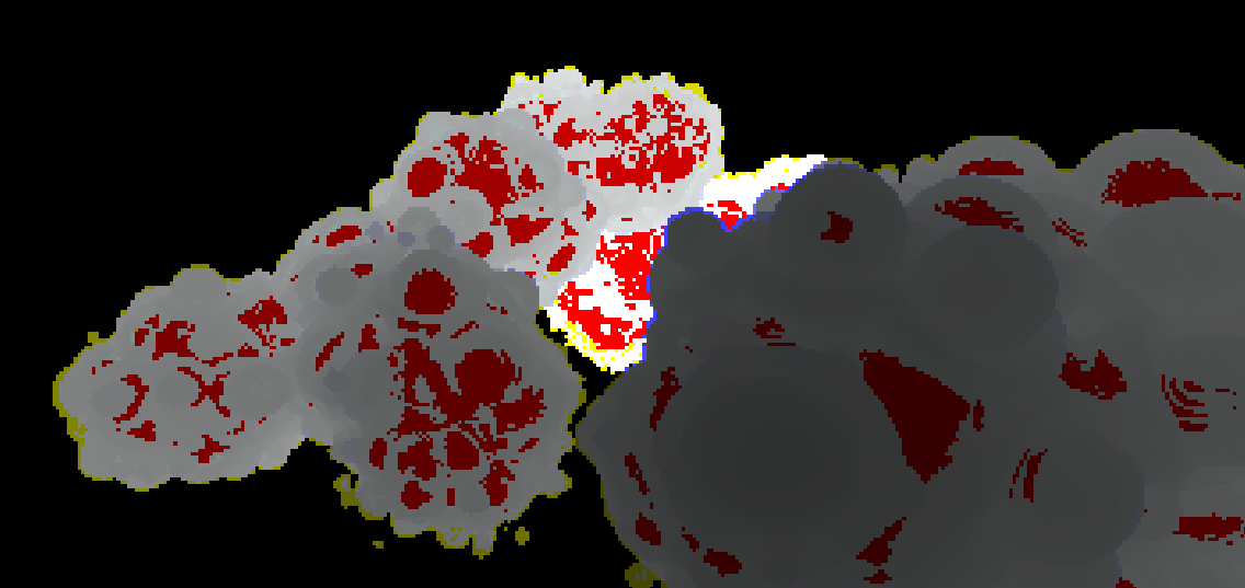
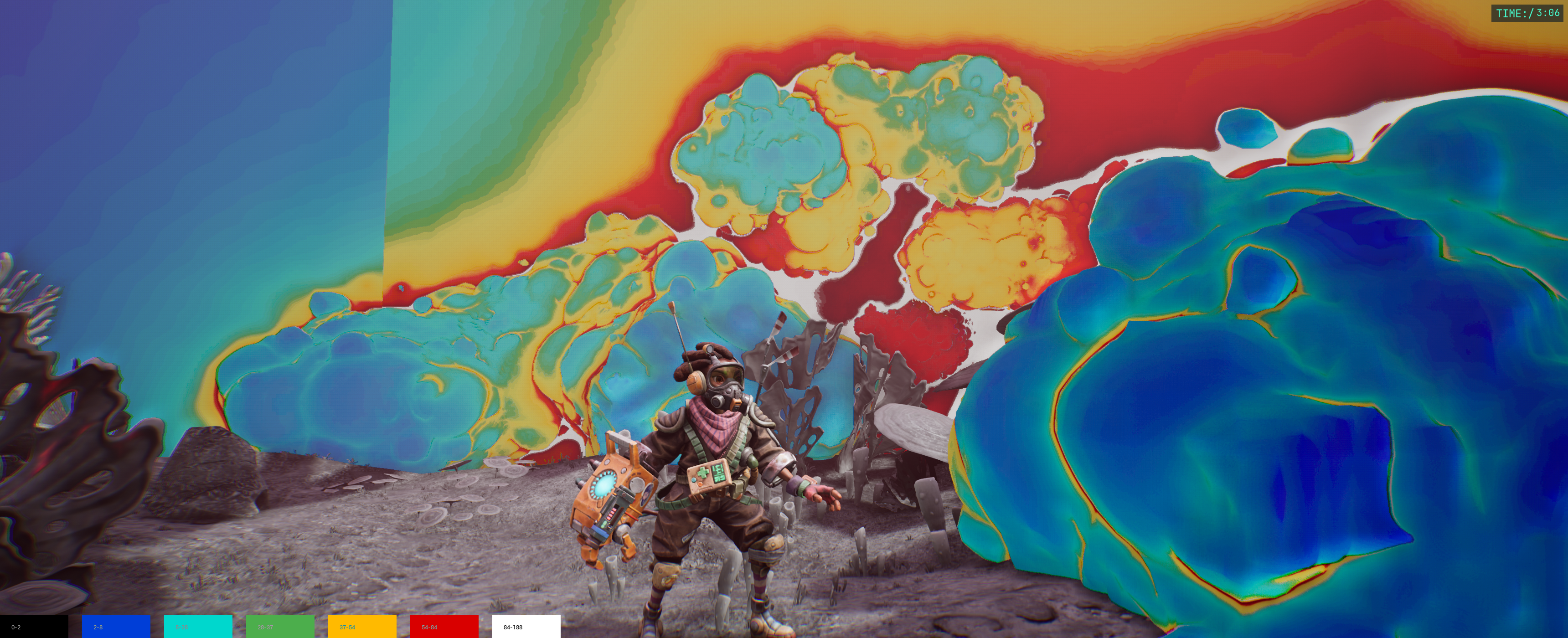 6.6 ms @ 4K
This is the cost of just raymarching a gunk field at 4K. In the image above we render the amount of steps as a heatmap. The warmer a pixel’s colour is, the more it costs us. As you can see a lot of expensive pixels render just empty space (even with AABB tests), so it is a lot of cycles down the drain.
6.6 ms @ 4K
This is the cost of just raymarching a gunk field at 4K. In the image above we render the amount of steps as a heatmap. The warmer a pixel’s colour is, the more it costs us. As you can see a lot of expensive pixels render just empty space (even with AABB tests), so it is a lot of cycles down the drain.
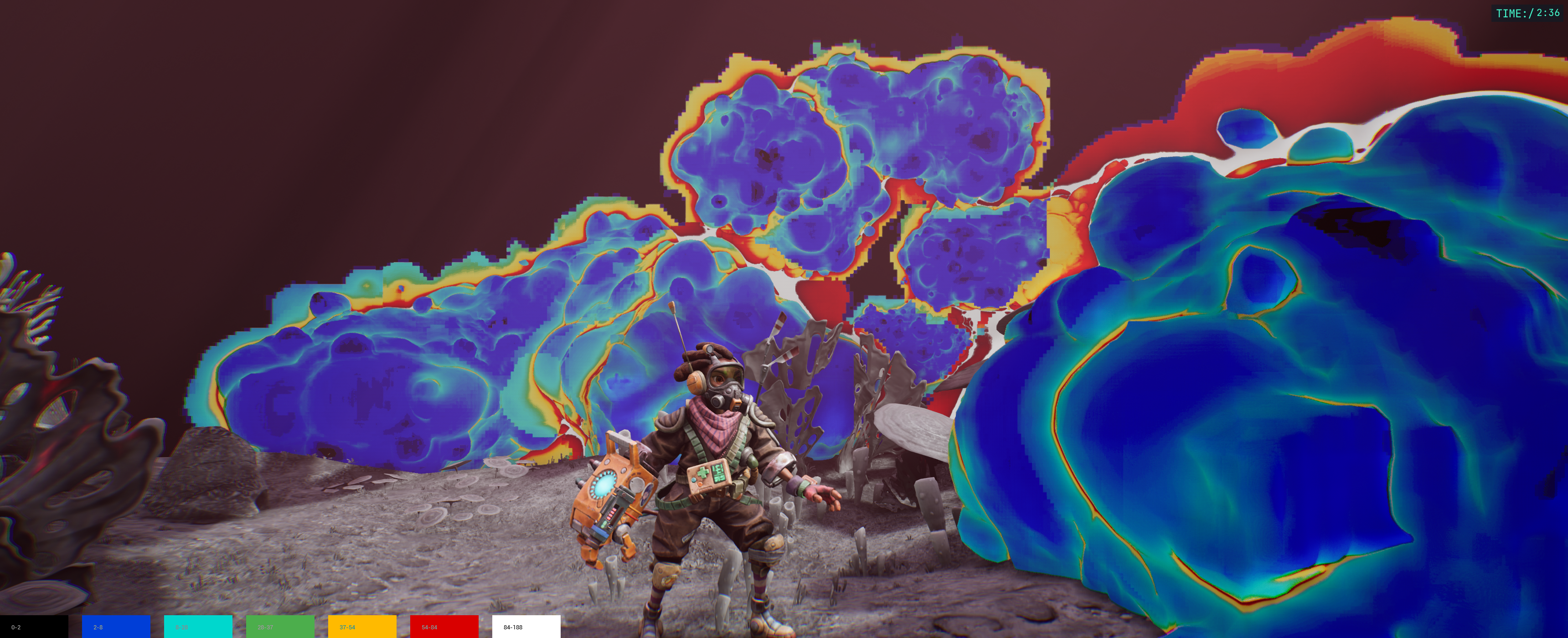 4.0 ms @ 4K
Using the conetracer pre-pass we are able to shave 2.6 ms of that time for that frame and completely avoid stepping in large parts of empty space.
4.0 ms @ 4K
Using the conetracer pre-pass we are able to shave 2.6 ms of that time for that frame and completely avoid stepping in large parts of empty space.
Total Frametime for raymarching passes and setup:
- 4 ms @ 4K on Xbox Series X
- 10 ms @ 1080p on Xbox One
Dynamic resolution scaling is then used for the final stretch of reaching our target framerates, and all screen buffers for gunk rendering scale to fit the dynamic resolution as well. Just as Unreal’s built in dynamic resolution this is achieved by changing the size of the rendered image (but not the buffer itself) and then applying the inverse scale on the surface on which it is rendered to screen.
Custom shadow rendering
The shadows cast by gunk are also raymarched, from the light point of view, to a custom depth buffer which is integrated in Unreal’s cascaded shadow pass. This is the work of Tim Sjöstrand! A true feat to dive into the depths of Unreal shadow rendering code and get all those moving parts to work!
Our early prototype for shadow rendering that I threw together for our announcement trailer was a glorious hack. It still rendered the gunk from light POV but rendered its silhoutte to a masked plane far up in the sky that would then cast the shadow onto the world, it worked just well enough for a trailer...
GPU: Superimpose renders to GBuffer using material
The final rendered buffers consist of a normal texture, a depth texture, and a mask texture. These are all fed into the material that is drawn over the whole screen as a fullscreen quad in Unreal’s basepass.
We employ some hacky solutions to do this in the simplest way possible. The fullscreen quad is a regular static mesh with large bounds that calculates the model view projection inverse as a vertex world position offset in the material, which causes it to always cover the full screen (be careful of floating point errors when doing it this way). Here the dynamic resolution is also applied as a world position offset.
The depth texture from the raymarcher is applied as a pixel depth offset to give the fullscreen quad correct per pixel depth. Pixel depth offset is applied with incorrectly angled vectors in Unreal 4’s materials, which causes some lookups (for instance indirect light volume) to become wrong on offset pixels. We thus change how pixel depth offset is applied so it is done in the correct space. This bug only really affects cases like ours where we work with the whole range of the screen and frustum and require each pixel to get a correct world position.
// MaterialTemplate.ush : ApplyPixelDepthOffsetToMaterialParameters

...

// Update positions used for shading
// Screen position is for example used for sampling decal buffer
// Transform to NDC to make new screen position given new depth (world scale to normalized scale)
const float2 NDC = MaterialParameters.ScreenPosition.xy / MaterialParameters.ScreenPosition.w;
// Add the offset to W, which is same as Viewspace Z
MaterialParameters.ScreenPosition.w += PixelDepthOffset;
// Reverse perspective divide to new screen position for new depth (now in world scale again)
MaterialParameters.ScreenPosition.xy = NDC * MaterialParameters.ScreenPosition.w;
MaterialParameters.SvPosition.w = MaterialParameters.ScreenPosition.w;
MaterialParameters.AbsoluteWorldPosition += MaterialParameters.CameraVector * PixelDepthOffset;
// Use screen-to-world matrix to transform to world space coordinates.
// This matrix leaves Z unchanged when unprojecting perspective, so use Screen W directly as Z.
// Absolute world position is for example used to sample indirect lighting volume
MaterialParameters.AbsoluteWorldPosition = mul(float4(MaterialParameters.ScreenPosition.xy, MaterialParameters.ScreenPosition.w, 1), View_ScreenToWorld).xyz;
Pull Request. This tweak fixes the offset to be in the correct space.
The surface normals are supplied from the rendered normal texture.
The mask texture contains different masks in its channels which we can use to mask in and out different colours and detail textures based on crevices and shapes.
With this setup we can control the full surface look of the gunk with a material graph.
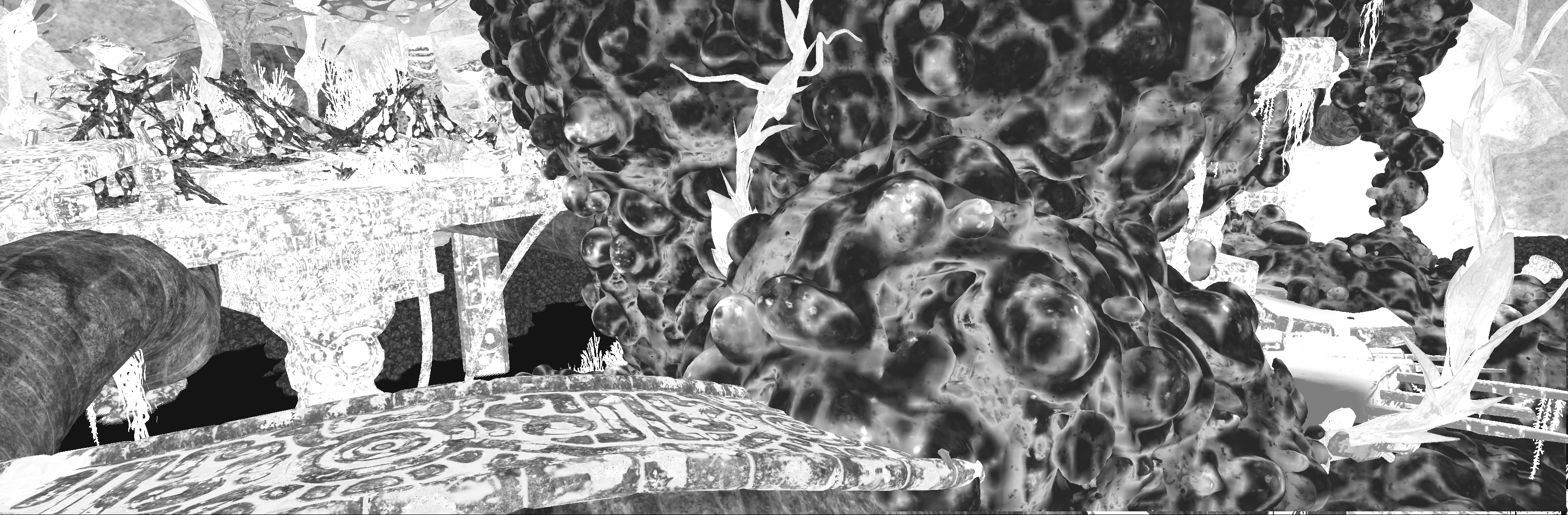
 Final scene composite
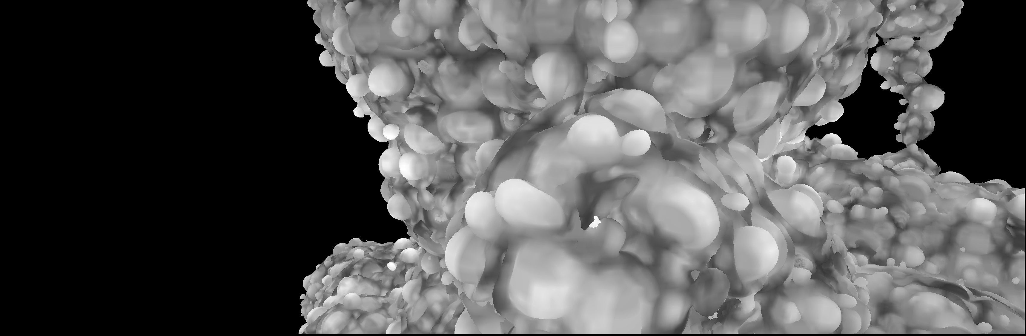
 Depth texture
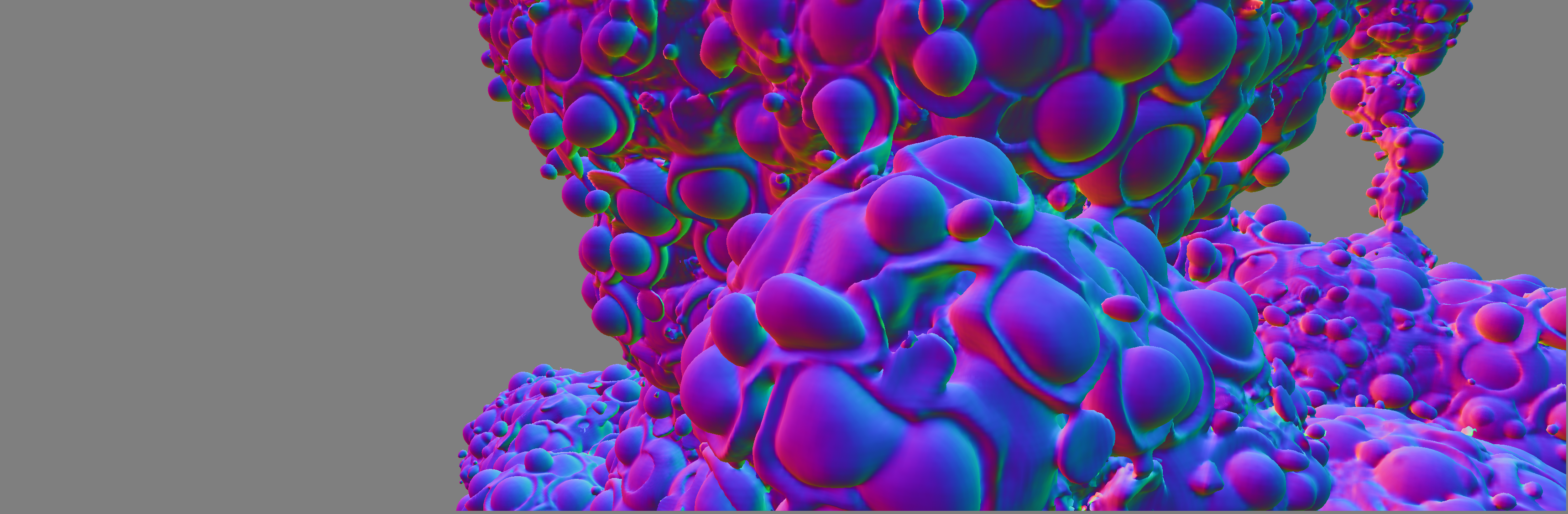 World normals
 Surface ramp mask
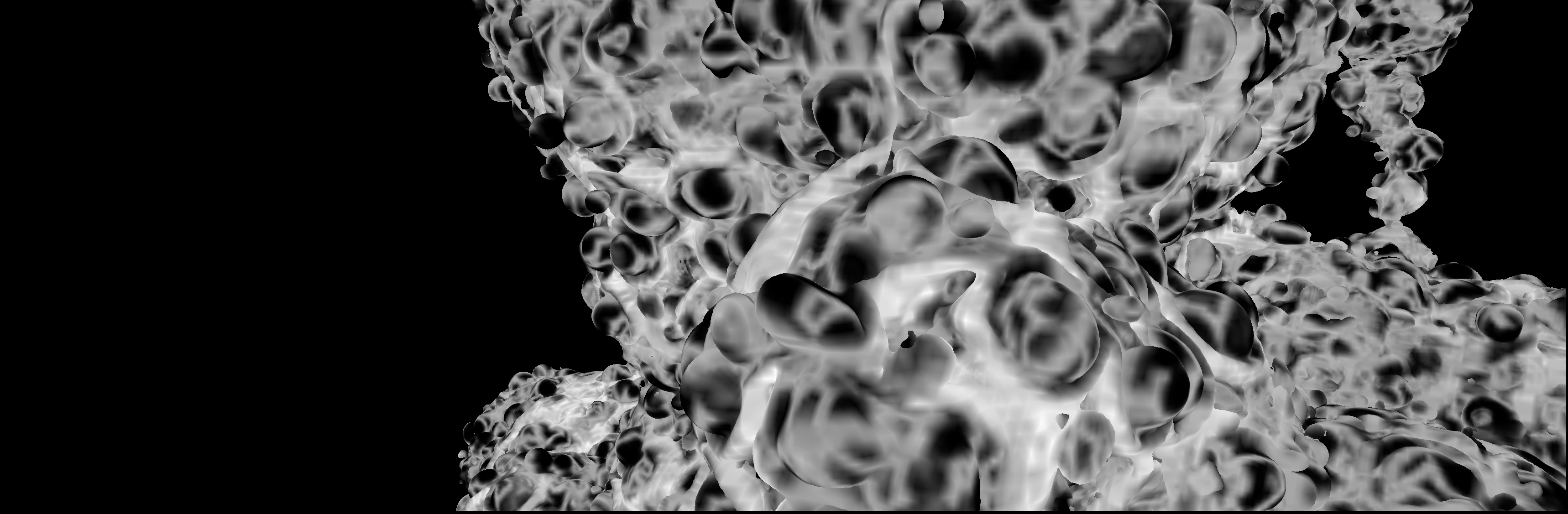
 Surface crevice mask
The material also makes use of low resolution-, tiling- and scrolling volumetric noise for detail roughness and normals. These are also masked with the rendered ramp- and crevice masks.
 Roughness channel with applied detail roughness texture.
 World normals with applied detail normal texture.
Frametime for fullscreen quad material:
- 1.4 ms @ 4K on Xbox Series X
- 2.7 ms @ 1080p on Xbox One
Unreal Engine integration
In order to be able to execute our compute shaders at custom points in the Unreal render pipeline we made a custom plugin and some changes to the engine.
The game thread sends per frame data to the renderer object that queues the data of draw parameters that the render thread then dequeues and reads. Both threads work with their own copies of the data, so this is the only point of lock and synchronisation.
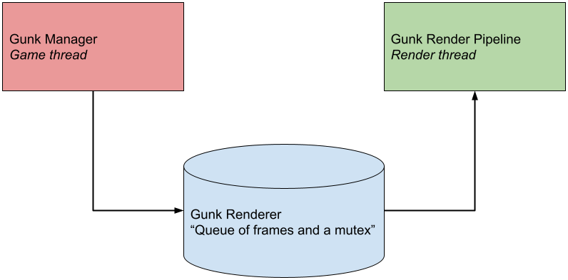 Overview of the plugin layout and communication between game- and render thread.
View information is fetched from the FViewInfo struct of the frame in the render thread so that the rendered perspective of gunk is in sync and exactly the same as that of the rendered frame.
In the render thread we try to use the main Render Dependency Graph (RDG) of the main pipeline to avoid unnecessary flushes between our code and Epic’s. My colleague Tim Sjöstrand did some stellar work porting my first version of the render pipeline to RDG. Previously all barriers were explicit and tracked in an Excel spreadsheet! Unfortunately not all parts of the pipeline are ported to RDG in Unreal Engine 4. As of Unreal Engine 5 the whole pipeline now uses it. But in Unreal Engine 4 the depth prepass still uses manual render commands and transitions. We wanted to run some of our compute shaders on the async pipe on platforms that supported it to win a couple of milliseconds in some cases. So in order to make that possible (without porting the prepass to RDG, which was out of scope for us), we changed where Unreal runs the main shadow depth pass, so it is run before the depth prepass. That way we could run some parts of the raymarcher in parallel to shadow rendering. We still incur a flush if the raymarcher takes longer than the current shadows, as we hit the prepass and have to wait.
Summary
So, in this article I tried to break down as many of the systems and steps that we made to realize the goopy gunk in The Gunk. We implemented a custom render pipeline alongside Unreal’s own, and we also made changes to Unreal so our custom passes can run in async compute to the built in shadow passes. This custom pipeline is used to render raymarched surfaces generated from voxels that the player can interact with. The custom pipeline converges into the regular render pipeline to allow us to use materials for the surface and get lighting from Unreal's existing lighting passes. With this solution we could have malleable blobs of gunk as a gameplay element and as a visual selling point of the game.
The Gunk was Image & Form's first Unreal Engine game. Getting all of it working for our small team was pretty crazy. The team pulled off a lot Herculean feats and I want to end this article by mentioning- and thanking my amazing teammates at Image & Form, The Station and Thunderful that I got to work with in this project and also to our contacts at Microsoft for all their help! And a big thanks to all the players who played our game!